Sphere lab
Scientific supervisor is Marc van Wanrooij
Introduction

The auditory sphere lab, located in the Huygens basement (at A -2), contains more than 100 high-quality speakers that are mounted on an acoustically transparent wire frame, allowing us to present a sound source at many different locations around the subject. In the middle of the sphere is a chair where a person (the subject) can sit, so that his/her head is exactly in the center of the sphere. Each speaker also has a small LED, which can provide a well-defined visual stimulus. We measure eye-head orienting responses of subjects to study sound-localization performance to well-designed acoustic stimuli, as well as audio-visual spatial behavior under a variety of spatial-temporal disparities. The lab is equipped with a high-end binocular eye tracker system (EyeSeeCam), with which eye movements can be recorded at 500 Hz sampling rate per eye.
For whom?
The equipment can also be used to test auditory spatial perception of patients with an implant, such as a cochlear implant, hearing aid devices, or a bone conduction stimulator. Companies producing such implants could gain more insight into the manner in which their products steer brain activity and perception. Audiological centers can use this technique for the same reasons.
The Sphere setup is a sound boot with about 130 speakers arranged in a sphere. The subject can be presented with stimuli in the form of sounds or led flashes. The head movements of the subject can be tracked. The subject can also respond to stimuli by pressing a button. The experiments are controlled by a computer and electronics from outside the boot.
The lab is located at the underground corridor (floor -2) between the Huygens Building and the Goudsmitpaviljoen (NMR). The entrance from the corridor is has the number W36A -2.002a. The Lab itself has the number -2.002d.
Experimental information
TDT programming
Basic information on TDT programming can be found in the RPvdsEx manual For everyone: read this first! (several examples: tones)
Basic sound localization experiment software
A basic sound localization experiment consists of several software components:
- xxxxxx.rcx for sound generation and data acquisition using TDT
- xxxxxx.m to input parameters, acting as a GUI
Sound generation
With the TDT system we can create and control sound stimuli in realtime. Stimulus parameters such as loudness, duration and onset timing can be controlled using the circuit components of the RPvdsex software. To create a stimulus, a relevant circuit has to be loaded onto the RP2 Realtime Processing unit. These files are called .rcx/.rpx files and can be found on the C:\MATLAB\experiment\RPvdsex drive on the experimental pc in the Biophysics lab.
Let's start with an example of gaussian white noise to see what is needed to present a stimulus.
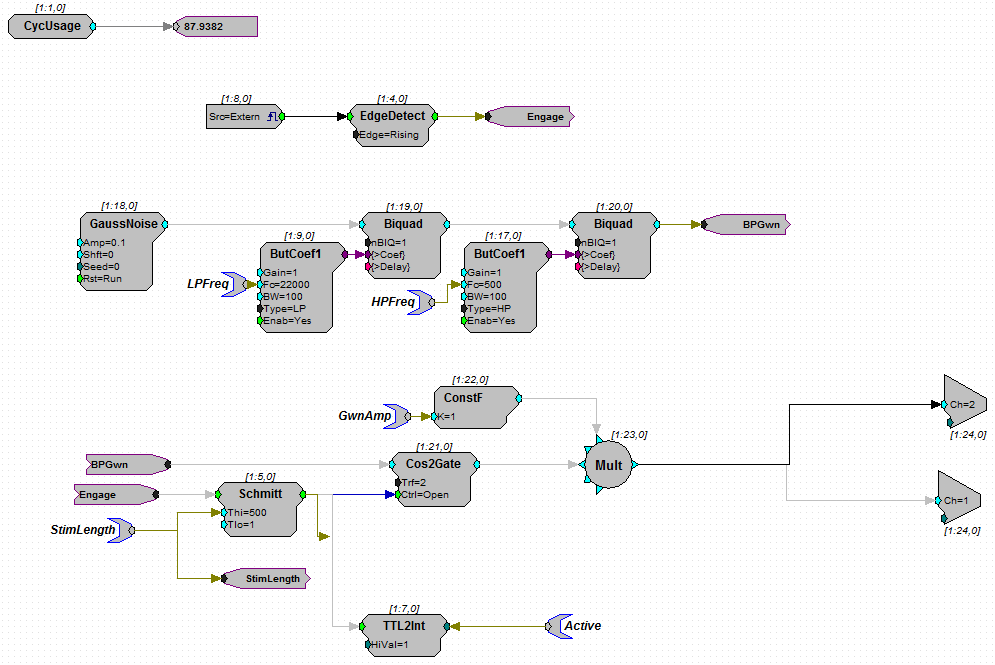

In the circuit shown above, we can see that there is a separate component called "GaussNoise". This generates random numbers that can be used to produce whitenoise through a speaker. After the GaussNoise component, there are two "Biquad" components in serie. The Biquad components both have input from "ButCoef1"; Butterworth filter coefficient generators. The result is a sound that is Lowpass filtered with cutoff frequency "LPFreq" and highpass filtered with "HPfreq". Both LPfreq and HPfreq are so called parameter tags, wich can be controlled via matlab with the command RP2.SetTagVal('HPfreq',MatlabHPfreq) where MatlabHPfreq is the Matlab variable with the value you want to assign to HPfreq in the circuit.
The filtered noise signal is passed to "BPGwn" (bandpassed Gaussian White noise) which is a simple linker component to create a clear flow in the circuit. The BPGwn reappears in the lower left part of the circuit, where it functions as input for a gating component "Cos2Gate". The gating component makes sure that the signal onset is a smooth transition from 0 to maximum amplitude, to prevent highfrequency onset artefacts. The Cos2Gate has additional green input in the form of Ctrl=Open, meaning that this is a digital (0 or 1) value. Likewise, the main input of Cos2Gate is light blue, meaning that it is a floating point value. When you create and compile your own circuits, the software checks if the input type matches the type of signal you connected. The Ctrl=Open port gets its input from the "Schmitt" component which creates a digital pulse of length "Thi" milliseconds. This is the stimulus duration, which you can change by altering the "StimLength" tag value. The Schmitt pulse is triggered by a linker called "Engage" which you can trace back to the top of the circuit. There and "EdgeDetect" looks for sharp positive change in the external trigger labeled "Src=Extern". This is the trigger input on the RP2 machine, usually you connect a button that the participant presses.
The output of the Cos2Gate is multiplied by "GWNAmp" to create a fixed loudness change. Note that you can also change the loudness by altering the "Amp" parameter in the GaussNoise component. After the multiplier, there are two components called "Ch=1" and "Ch=2". These are Digital to Analog Converters (DAC outputs) and they correspond to the two output channels on the RP2.
After the RP2, the sound signal is led through a PM2relay ("MUX machines" or Multiplexers) to assign which speaker should present the sound.

In this part of the circuit, we will start with the output instead of the input. Output here is the "WordBitOut" on the right with "M=-1" written inside. The wordbitout is a digital output with 8 bits. From the TDT system manual: Bits 0 - 3 identify the channel number. Integer 0, or bitpattern (xxxx 0000), is channel 0 and integer 15, or bitpattern (xxxx 1111), is channel 15. Bits 4 and 5 identify the device number. Integer value 0, or bit pattern (xx00xxxx), is device number 0 and integer value 48, or bit pattern (xx11xxxx), is device number 3. The device number is set internally for each PM2R and allows for an RP2 to control up to four PM2R modules. If only one PM2R is being used, it should have device number 0. Bit 6 is the set-bit. When this bit is set high, the channel and device from the previous six bits is activated. Bit 7 deactivates all channels across only the specified device.
This means that you need to add several integer values to switch on the speaker you want. To select the channel (0-15) on a multiplexer, you can change the "GwnChan" tag. To select a multiplexer device, change the "DeviceSelect" tag value. Finally, to switch on the selected speaker, choose value 64 for "SetReset" and trigger the software trigger (the "Src=Soft1" component) via matlab. To know which speaker (azymuth, elevation location) belongs to which configuration of multiplexerindex and channel, use the SoundSpeakerLookUp function in matlab (more on this function and other matlab functions in another section).
Timing of sounds The timing of sound playback is an important factor in an auditory experiment. Humans can detect onset differences at millisecond level, so knowing when your sound was presented and when it ended is crucial for analysis. A specific part of the sound presentation RP2 circuit is designed to measure and store onset/offset timings for sounds. This part of the circuit is shown in the figure below:

The timings of sound onset and offset are based on the change in WriteSound. Once SoundOn or SoundOff is high, the Schmitt2 sends a single sample pulse to the SerStore buffer component. The buffer stores the value in the Counter (the Clock value). The counter can be set at any time before stimulus presentation, because only the relative timings between different events in a trial (button presses, LED timings, data acquiring) matter. In the circuit above, the counter is switched on with a zBusA trigger. This has the advantage that multiple circuits on different machines can be triggered simultaneously. The tags OnsetTimings and OffsetTimings can be read using the matlab command RP2.ReadTagV('OnsetTimings',0,1) (or 'OffsetTimings').
Recording headcoil data with TDT system
The data we measure in our localisation experiments are voltage changes in the headcoil that participants wear. A head movement results in a change in flux through the headcoil and thus in a different magnetic induction current for all three (horizontal, vertical, frontal) magnetic fields. This raw voltage signal is led through the Remmel system, which demodulates the signal into three separate signals for the three orthogonal directions.
These three signals are amplified by the RA8GA Adjustable Gain Preamp. The "Range Select" of this machine should always be on 10V. The amplified signal is passed onto the RA16 Medusa Base Station. The RA16 collects the data and a specifically designed .rpx circuit can provide a readout that can be saved in a Matlab environment.
The data on the RA16 is stored in internal buffer units, that have to be controlled via a Matlab initiation. Let's take a look at the circuit to understand how data is recorded and exported:
An important aspect of the design is the timing of the signal aqcuisition. Ideally, you want the acquisition to start at the same time that the sound stimulus from the RP2 is played. This is implemented by using a zBus trigger that is used by both the circuits in the RP2s and in the RA16.
Storing data
Data from the localization experiments should be stored in a HDF5 file. This file should hold all information about the experiment. A matlab function is availabe to write your .mat data into a HDF5 file.
the structure of this file is as following:
 /ExperimentInfo (date, time, experimenter, subject number, experiment type, session number)
 /StimulusInfo   (stimulus type, stimulus parameters, hardware settings, used TDT circuits or wav-files)
 /TrialLog       (per trial information: single trial stimulus parameters (LED/Sound) onset/offset, buttonpress timing, data readout timing)
 /HeadMovement   (headcoil readout channels)
 /Notes          (additional information; participant comments, abnormalities)
With the HDF5 file format, you can write multiple sessions with the same participant in the same file, so you won't have to edit all the metadata everytime you save a new session.
Running a localization experiment
<todo>